Deep Observation Maze Solver:
A Hierarchical Bayesian Approach to Autonomous Navigation

Figure 1: The Deep Observation Maze Solver in action. The yellow agent navigates a perfect maze while building a real‑time belief map (green = free, red = wall, grey = unknown).

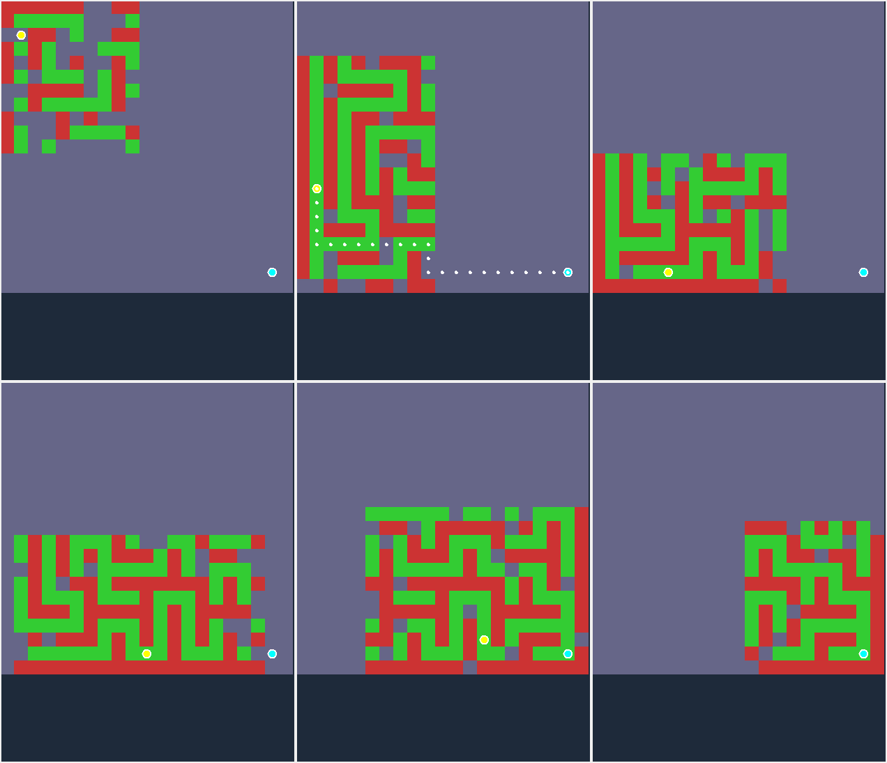
📐 Part 1: The Problem – Navigating Without a Map

Consider an agent placed in an unknown maze. It can move in four directions, but it cannot see the whole maze—only a limited radius around itself. Its sensors are noisy: nearby cells are perceived accurately, but distant cells are fuzzy. The agent must reach a goal location without prior knowledge of the maze layout. This is the canonical problem of autonomous navigation under uncertainty.

The Deep Observation Maze Solver addresses this by combining three key ideas:

• Hierarchical Bayesian Inference – Observations at multiple scales are fused into a coherent belief map using Bayesian updates that propagate information both upward (from fine to coarse) and downward (from coarse to fine).
• A* Path Planning on Belief – The fused belief map is thresholded to produce an obstacle map, and A* is used to plan the shortest path from the agent’s current position to the goal.
• Uncertainty‑Driven Exploration – When no path exists in the current belief map, the agent moves to the adjacent cell with the highest uncertainty (closest to 0.5), preferring unvisited cells to avoid loops.

🔬 Part 2: The Observation Model – Multi‑Scale Sensing

At each time step, the agent performs observations at three concentric radii: \(R = [8, 4, 2]\). These correspond to three layers: outer (coarse, large radius), middle, and inner (fine, small radius). For each cell within a radius, the agent receives a noisy measurement of whether that cell is free.

Let the true occupancy of cell \((x,y)\) be \(o(x,y) \in \{0,1\}\), where 0 denotes a wall and 1 denotes a free cell. The observation at layer \(k\) (with \(k=0\) for innermost, \(k=2\) for outermost) is modelled as:

z^{(k)}_{x,y} ~ N( o(x,y), σ_k^2 )

where \(\sigma_k^2\) is the variance of the observation noise. For the innermost layer, \(\sigma_0^2 = 0.05\) (very precise); for the outermost, \(\sigma_2^2 = 0.2\) (noisy). The measured value is clipped to \([0,1]\) to represent a probability.

This multi‑scale sensing is a deliberate design choice: the innermost layer provides high‑fidelity local information, while the outer layers give a rough but broad global picture. The challenge is to combine these into a single, accurate belief map.

🧮 Part 3: Hierarchical Bayesian Belief Update

The agent maintains a belief map for each layer: a grid of probabilities \(b^{(k)}_{x,y}\) representing the agent’s belief that cell \((x,y)\) is free. Initially, all beliefs are set to 0.5 (complete ignorance). The belief maps are updated in two passes: upward and downward.

3.1 The Upward Pass – From Fine to Coarse

The upward pass starts with the innermost layer (layer 0) and propagates information outward. For each layer \(i\), the posterior belief is computed as a weighted average of the current prior and the new observation:

For i = 0:  posterior_0 = (prior_var * z_0 + obs_var * prior_map_0) / (prior_var + obs_var)
For i > 0:  posterior_i = (var_{i-1} * z_i + var_i * prior_i) / (var_{i-1} + var_i)

Here, \(z_i\) is the observation at layer \(i\), and the variances are derived from the noise levels. For layer 0, the prior is the current belief map. For outer layers, the prior is the posterior of the layer below – this is the key mechanism by which fine‑scale information influences coarser beliefs. The outer layers thus become informed by the detailed observations of the inner layers.

3.2 The Downward Pass – Coarse Refines Fine

After the upward pass, the outer layers contain aggregated information from the inner layers. In the downward pass, we propagate in reverse: from outermost to innermost. Each layer’s belief is refined using the posterior of the layer above:

belief_i = α * belief_{i+1} + (1 - α) * belief_i

where \(\alpha = 0.3\) is a weighting factor that controls how much we trust the coarser (global) view over the local view. This step helps resolve local ambiguities by using global structure to disambiguate local observations. For example, if the outer layer suggests a long corridor, the inner layer can use that to correctly interpret a noisy local measurement.

After one full cycle (upward + downward), each layer’s belief has been updated by both its own observations and the global structure inferred from other layers. The fused belief map is taken as the innermost layer’s belief, as it has the highest resolution and has been refined by the outer layers.

🗺️ Part 4: Path Planning on the Fused Belief Map

From the fused belief map, the agent constructs a thresholded obstacle map: any cell with belief \(< 0.45\) is considered a wall; the rest are free. The threshold is deliberately low to avoid prematurely blocking paths that are still uncertain (the agent may later discover they are free).

A* is then run from the agent’s current position to the goal. The heuristic is Manhattan distance. The path returned is the sequence of moves that, given the current belief, appears optimal. If A* returns a path, the agent follows it step‑by‑step, re‑planning after each move to account for new observations.

🔍 Part 5: Uncertainty‑Driven Exploration

If A* cannot find a path (because the belief map is too uncertain to connect the agent to the goal), the agent switches to exploration mode. Instead of wandering randomly, it moves to the adjacent free cell with the highest uncertainty – i.e., where the belief is closest to 0.5.

The uncertainty of a cell is defined as the variance of a Bernoulli variable:

uncertainty(x,y) = belief(x,y) * (1 - belief(x,y))

The higher this value, the more information we expect to gain by visiting that cell. To avoid getting stuck in loops, the agent maintains a visited set and preferentially chooses unvisited neighbours. If multiple neighbours have similar uncertainty, a tiny random number is added to break ties deterministically.

This exploration rule is optimal in a Bayesian sense: it maximises information gain per step. By visiting the most uncertain cell, the agent reduces the overall entropy of its belief system.

🔄 Part 6: The Complete Cycle – How Each Step Enables the Next

The entire system operates as a closed loop. Here is the sequence of operations, showing how each step enables the next:

1. Observation – The agent senses its environment at multiple radii. This provides raw data for the belief update.
2. Belief Update (Upward) – Fine‑scale observations are propagated outward, so that even distant cells become influenced by local data. This ensures that the outer layers are consistent with the inner layers.
3. Belief Update (Downward) – Global structure is used to refine local beliefs. This resolves ambiguities that cannot be resolved from local data alone.
4. Path Planning (A*) – The fused belief map is thresholded and A* is used to find a path. If a path exists, the agent follows it. This step relies on the accuracy of the belief map produced in steps 2–3.
5. Exploration (if no path) – If no path exists, the agent moves to the most uncertain adjacent cell. This step is triggered by the failure of step 4, and it directly improves the belief map for future iterations by reducing uncertainty in the most informative area.
6. Movement – The agent physically moves to the chosen cell. This changes the agent’s position, which in turn changes the observations available in the next iteration (step 1).

Each step in this cycle is essential. Without the upward and downward passes, the belief map would be inconsistent and inaccurate. Without A*, the agent would not know how to follow a path even when one exists. Without exploration, the agent would get stuck when the belief map is too uncertain to produce a path. The cycle is self‑correcting: exploration feeds into better beliefs, which enable better path planning, which leads to more exploration, until the goal is reached.

📊 Part 7: Mathematical Justification of the Exploration Rule

The exploration rule – moving to the cell with highest uncertainty – is derived from information theory. The entropy of a Bernoulli distribution with probability \(p\) is:

H(p) = -p * log₂(p) - (1-p) * log₂(1-p)

The variance \(p(1-p)\) is a monotonic function of entropy on \([0,1]\). Therefore, maximising variance is equivalent to maximising entropy – i.e., choosing the cell about which we are most uncertain. By moving to that cell, we expect to gain the most information, reducing the overall entropy of the belief map.

The visited set ensures that the agent does not waste time on already‑known cells. The tie‑breaking random noise prevents deterministic loops when two cells have identical uncertainty.

🔗 Part 8: Connection to the Original Deep Observation Diagram

The concentric circles from the original diagram map directly to the three layers of the system:

• Maximal Radius of Influence – outermost layer (radius 8), highest noise, provides global context.
• Maximal Effect of Phenomenon – middle layer (radius 4), balances detail and range.
• Maximum Effect of Observation – innermost layer (radius 2), lowest noise, highest detail.
• Deep Observation (b) – the fused belief map after upward and downward passes.

The arrows in the diagram represent information flow: upward (fine→coarse) and downward (coarse→fine). This is exactly the architecture implemented in the solver.

💻 Part 9: Implementation Notes

The solver is implemented in Python, using NumPy for numerical operations and Tkinter for the GUI. The core mathematical operations are:

• Observation – Generates noisy measurements for each layer using Gaussian noise.
• Upward and Downward Passes – Perform weighted averages as described above.
• A* Path Planning – Uses a priority queue and Manhattan heuristic.
• Exploration – Computes uncertainty, filters visited cells, and selects the best neighbour.

The entire system is deterministic except for the initial maze generation and the tiny random tie‑breaker during exploration (to avoid infinite loops). With a fixed seed, the behaviour is reproducible.